SECTION 49
GALACTIC NOISE EXPERIMENTS - PART 2
(June 30th, 2016)
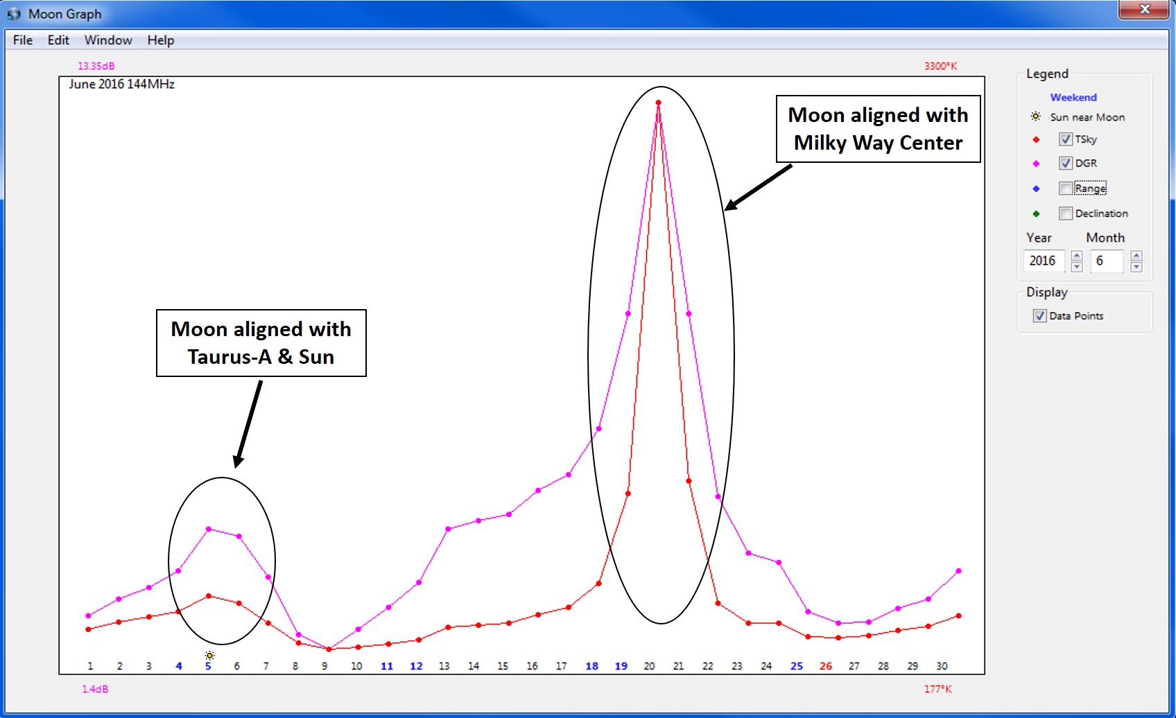
PS: to the right, a picture of the Moon Graph for the month of June, which shows the Sky Temperature (red curve) and the EME Degradation Factor (pink curve).
The experimental work presented in Section 46 provided me some initial data which helped showing how much the Milky Way was affecting the noise level and also helped revealing the "diffuse nature" of it (Sky filling). The diffuse nature attribute is actually mentioned in the EME Handbook (2010) under the section "Background Noise". I only found that out after the fact which helped confirming my own observations. http://physics.princeton.edu/pulsar/K1JT/EME_2010_Hbk.pdf
Looking at a typical TSky/DGR Moon Graph (picture to the right), it is clear that the EME Degradation Factor (DGR) is highly driven by two main events, i.e. when the Moon is almost and/or perfectly aligned with the Center of the Milky Way ans same with Taurus-A but to a much lesser extent. The Sun can also add significant noise as shown in Section 47. The Moon Distance also affects DGR, up to a max of about 2.2dB compared to when Moon is the closest to earth.
Here is how the EME Degradation Factor is calculated based on what I found on the internet:
Degradation [dB]: Degradation in EME signal-to-noise, calculated as: Tsky [K] / (TskyMin [K] + Tsys [K] ) + RangeFactor [dB]
Moon distance [km]: Earth-Moon distance. Mean distance is 384400 km. Minimim during perigee 356400 km. Maximum during apogee 406700 km. This translates to as much as 2.25dB difference in pathloss from apogee to perigee.
Moon declination [deg]: Moon declination in degrees north (+) and south (-) of the equator. Max declination up to 28.7 degrees.
Calculation assumptions for 144MHz: TskyMin = 200 K, Tsys = 80 K, Observer Position = Central Europe, Time = 12:00 UTC, Tsky data interpolated from EME Handbook 2010 / WSJT 7.03 source data by K1JT.
Conditions summary: Conditions are summarized on basis of the degradation. Be aware that this is only a theoretical approach and the real conditions may vary due to local or ionospheric changes. In general this info is only meant to show the current astronomical situation and to indicate a global trend. Within a day of New Moon (NM), high sun noise can make conditions 'Very Poor' regardless of the DGR. The conditions are classified i.a.w. following DGR [dB]:
< 1.5 => Excellent
> 1.5 and <= 2.5 => Good
> 2.5 and <= 4.0 => Fair
> 4.0 and <= 5.5 => Poor
> 5.5 => Very Poor
After I found out how the Degradation Factor was calculated, I quickly started questioning the applicability of it for various QTH where based on the calculation assumptions above, the "position observer" is in Central Europe at 12 UTC. The Sky temperature at that QTH may be significantly different compared to other QTH. Based on my own experiments, it was clear that the Milky Way for instance had to be a dominant factor in the Sky temprature as shown in the Moon Graph above. The problem is that above ~62 degrees North Latitude for instance, the Milky Way NEVER rises above the Horizon! To the contrary, in Sydney Australia for instance, the Center of the Milky Way may reach elevations as high as 85 degrees above the Horizon. Obviously, the Sky Noise figures and corresponding DGR between these different extreme cases/QTH have to be quite different. Based on that alone and the fact that DGR calculated by WSJT is the same regardless of the QTH of an EME station, one has to be very careful in its use and interpretation.
I later found an interesting posting by the author of WSJT himself:
"...Never take any number like these "Dgrd" values as gospel, without thinking about what it means and how it was computed. Briefly stated, we want a number that characterizes how much "worse" EME conditions are, when the moon is in different locations. To calculate such a number, you'd need to know the Rx noise figure, the antenna main-lobe width, the sidelobe responses, the local noise situation, and many other details. A program can assume some supposedly "average" values, and make guesses for others, but they certainly won't apply to every setup. Differences in calculated values are especially large when the moon is close to the plane of the Milky Way galaxy, because antenna beamwidth then makes a big difference. Older versions of WSJT and MAP65 did not apply any smoothing (i.e., choosing a supposedly "average" antenna beamwidth) to the map of sky brightness temperatures. The current MAP65 v1.99 does this, assuming a 15-degree beamwidth. This tends to reduce the peak computed Dgrd values.
The bottom line: At best, a single Dgrd number is no more than a general indication that may be generally applicable for a fictitious, supposedly average, station."
Joe
The posting above only reinforced my conclusions. Therefore, instead of simply relying on these types of index, it became clear that quantifying the impact of the Milky Way based on my own setup and QTH using an emperical approach remained the best way to really get to the bottom of this and acquire the corresponding knowledge.
 QUANTIFYING THE INFLUENCE OF THE MILKY WAY
In order to further quantify influence of the Milky Way and better understand the diffuse nature of it, I thought about creating a map of the Sky by measuring the noise level at different AZ/EL while the Milky Way was: 1) below the Horizon. 2) At its peak above the horizon.
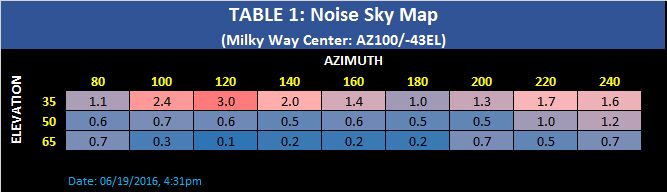
That is precisely what the results in Table 1 and 2 represent. For this particular experiment, I used a "Dummy Load" (instead of the antenna) to set the lowest noise level at 0.0 dB and then connected the array to perform the measurements at the different AZ/EL. The figures in the tables are in relative dB as measured by WSJT-10 in the measure mode.
 As shown in Table 1, when the Milky Way is below the horizon (AZ100/-43EL), the noise level is very low, that is near "Dummy Load" level. It is important to note that in Table 1, the noise measured at 100-120AZ/35 EL is significantly higher compared to the other coordinates in this table. This is mainly due to the fact that at these particular coordinates, the antennas are in very close proximity to the house chimney, which distorts the radiation pattern and let some more noise gets in.
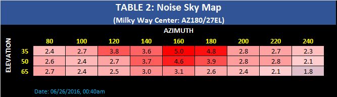
In Table 2, i.e. when the Milky Way is at its peak in the Sky of Southern California (AZ180/27EL), the noise level is much higher for ALL the coordinates measured, that is for the entire Sky being mapped out. These results were very interesting to me and really reinforced the conclusions about the diffuse nature of the noise produced by the Milky Way. It shows how much the entire sky can be "contaminated" and filed by the noise produced by our own Galactic Body. Generally speaking, looking at Table 2, the noise level is higher by about 2.5-3dB for all the coordinates measured compared to Table 1, and up to 4-5dB higher for the coordinates close to the actual Milky Way location. That is very significant in the world of EME!
TURNING DATA INTO INFORMATION
 In light of these results, the natural and logical conclusion suggests that the lowest Sky Noise level (best EME conditions) should occur when the Milky Way is below the horizon. Of course, one must still consider the other factors mentioned above such as Moon Distance, Sun presence, etc.
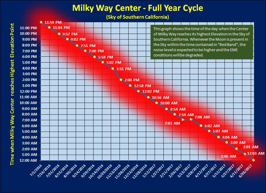
From there, I created a chart which shows the time of the day when the Milky Way is at its peak in the Sky of Southern California (my QTH) during 2016-2017. See picture to the right. The time contained within the "Red Band" represent the least favorable time for EME operation.
As one can see, over a period of a year, the Milky Way peaks at different time covering a full 24-hour cycle. For instance, looking at the chart, from 07/01/2016 to 09/14/2016, the corresponding evenings are likely to be quite "noisy" as the red band falls between 11:59pm and 7:00pm respectively (local time). The optimum time for EME operation being at any time falling in the "blue" portion of the graph. I now call this period the "Golden Hours"...:) Obviously, the Moon has to be present in the sky for EME to be possible in the first place.
After creating the graph to the right, I quickly made noise measurements to try to validate this theory. As I am writing this text (June 30th, 2016), I observed that the late evenings over the last many days have been extremely noisy and would NOT be favorable for EME operation based on the noise level alone. This makes perfect sense since the late evenings at this time of year fall within the Red Band, that is, when the Center of the Milky Way is heavily present in the Sky.
CONCLUSION
The recent experiments described in Section 46-49 really helped me develop a much better understanding of some key sources of Sky Noise and have a good feel of the magnitude of their potential impact on EME operation. That knowledge is precious to me since I can then utilize it to develop operational strategies and make the best out of my EME experience.
Stay tuned for more!